INTRODUCTION
There are many ways to identify an individual, depending on whether he is dead or
alive. Thus, more specifically for the identification of human skeletal remains,
a variety of methods can be used such as DNA analysis and teeth X- rays1,2. Although these methods provide valuable information for forensic
scientists in relation to age, sex and body size of the dead, many of them may
not be useful.
They depend on the availability of a comparative material, either from police
database, dentists or relatives, which can make identification impossible1,3. Facial reconstruction is the last process when identification
methods have failed2. Based on average
values of facial soft tissue thickness obtained in particular populations is
possible to obtain an image of an unknown dead, that may allow recognition of an
individual.
Detailed information obtained from physiological and osteological analysis of
remains such as sex, age, and thickness of soft tissue in a specific population
can promote the success of an identification. Data on the soft tissue thickness
represent an integral part of the paths to obtain similarity of a face4, assuming that cranial morphology is
sufficiently distinct and provides an efficient framework for a single facial
appearance even when applying average values of soft tissue thickness.
Recently, the number of studies on this subject has increased. Many established
methods measure thickness of soft tissues. To this end, some studies used
cadavers inserting a calibrated needle in distinct points of the face5-8. Some imaging techniques, used in living people, can minimize the
error caused by the soft tissue post-mortem changes when these studies are in
cadavers. Taking into consideration that each of these techniques have their own
advantages and disadvantages, it can be cited the following: radiography9-13, ultrasound3,14-19, magnetic
resonance imaging2,20,21, and computed tomography1,22,23.
Furthermore, previous studies have shown that different groups present
significant variation in soft tissue thickness, questioning whether data of a
population may be applied in facial reconstruction of another with different
ancestry2,7,10,11,16,24. For this
reason, for obtaining an accurate facial reconstruction, construction of a
database on soft tissue thickness of a particular population is required.
There are available data published in literature on soft tissue thickness
in vivo among Japaneses25, Portugueses8,
Egyptians16, Indians21, Zulus15, mixing of populations of South Africa23, African-americans26 and Greek14. Nevertheless,
for the Brazilian population there are studies only on cadavers9.
OBJECTIVE
This study intends to compose a database for determining soft tissue thickness
and begins with this pilot study, aiming a future facial three- dimensional
reconstruction of Brazilians to apply in recognition of skeletal remains as well
as to compare its results with other populations worldwide.
METHODS
The sample was estimated using the PC-SIZE 1.1 program (1990) by making use of
data source with variable similar to the article Panenková et al.1. The calculation was based on the
craniometric point malar lower in females and males. The mean and standard
deviation were used for this calculation. This variable had a significant
difference in the study and leaded to a larger sample compared to other
craniometric points also with significant differences. The total number of
patients was 101, with 0.90252 of power analysis and considering a 0.05
significance level.
This cross-sectional pilot research studied in a Brazilian North Eastern
Population, most precisely in Recife, state of Pernambuco. The sample comprised
of 101 patients’ images, who sought the radiological clinic of the University
Hospital Oswaldo Cruz/University of Pernambuco over a period of six months. For
this reason, patients have not been exposed to radiation only for research.
Exclusion criteria were patients with indications of trauma, congenital facial
disorders, skin edema, previous surgery or artifacts in CT. Participation was
voluntary.
The variables considered were sex, age, height and weight of each person, they
were collected at the same time of CT examination. The following formula
calculated body mass index (BMI): weight/height2 (kg/m²). According to others studies3,8,26, four BMI
ranges were considered: thin (BMI < 20); normal weight (BMI = 20-25); over
weight (BMI > 25). Ages were arranged into age groups 18-39, 40-59 and 60
years old or more.
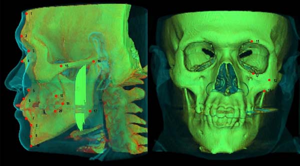
In this research, measurements of soft tissue were performed on 20 skull
anthropometric points (Table 1 and Figure 1). Many of which are standard points
most commonly used in the studies found in the literature22,26-28, ten are in
the midline and ten are bilateral. For anthropometric convention, only midline
points and the left ones were considered.
Table 1 - Description of craniometric points considered in this study
(Tedeschi-Oliveira et al.
8; Dong
et al.
22).
| Medium-sagittal Points |
Description |
| 1. Supra-glabella |
The most anterior point of the forehead, above the
glabella in the midsagittal plane
|
| 2. Glabella |
The most prominent point between the supra orbital
ridges in the midsagittal plane
|
| 3. Nasion |
Midline point on the internasal suture |
| 4. Rhinion |
The anterior tip of the nasal bones |
| 5. Midphiltrum |
Midline of the maxilla, placed as high as possible
before the curvature of the anterior nasal spine begins
|
| 6. Supra dentale |
Centered between the maxillary central incisors at
the level of the cementum-enamel junction
|
| 7. Infra dentale |
Centered between the mandibular central incisors at
the level of the cementum-enamel junction
|
| 8. Supra mentale |
Deepest midline point in the groove superior to the
mental eminence
|
| 9. Pogonion |
Most anterior midline point on the mental eminence
of the mandible
|
| 10. Menton |
Most inferior midline point at the mental symphysis
of the mandible
|
| Bilateral points |
|
| 11. Supra-orbital |
Centered upper part of the margin of the orbit |
| 12. Infra-orbital |
Centered lower part of the margin of the orbit |
| 13. Lateral orbit |
Lined up with the lateral border of the eye on the
center of the zygomatic process
|
| 14. Inferior Malar |
Lower part of the jaw |
| 15. Zygomatic arch |
Zygomatic arch the most lateral point of the
zygomatic arch
|
| 16. Supra-glenoid |
Root of the zygomatic arch just before the ear |
| 17. Gonion |
Point located on the jaw line at the level of the
angle between the posterior and the inferior borders of the
mandible
|
| 18. Supra M2 |
Point located on the alveolar process at the level
of the middle of the second upper molar (if this tooth loss, the
point is placed in the corresponding area)
|
| 19. Occlusal line |
Point located on anterior margin of the ramus of
the mandible, in alignment with the plane of dental
occlusion
|
| 20. Sub M2 |
Point located on the alveolar process at the level
of the middle of the second lower molar (if this tooth loss, the
point is placed in the corresponding area).
|
Table 1 - Description of craniometric points considered in this study
(Tedeschi-Oliveira et al.
8; Dong
et al.
22).
Figure 1 - Craniometric points.
Figure 1 - Craniometric points.
A multi-slice computed tomography / GE 4-channel with a thickness of 1.25 mm and
slice increment of 1 mm were used in the study, which can provide sectional
images in three planes and a three-dimensional object. The images were displayed
on InVesalius 3.0 program that provided an adjustment of the position and
orientation of head plans and shows skull and surface of the superimposed
face.
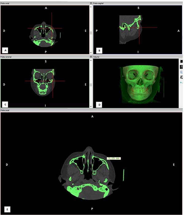
Measurements were taken perpendicularly to craniometric points according to
Vanezi et al.29). The length of facial
soft tissue thickness was measured by drawing a line perpendicular to a facial
skeleton point towards the soft tissue (Figure 2). The measurements were performed on the monitor using a CT console
cursor, with an accuracy of 0.01 mm. All data were recorded on appropriate
forms. Points’ description is presented in Table 1 and Figure 1.
Figure 2 - A: Positioning an anatomical landmark: lateral orbit
point (D13) in axial axis; B: Positioning an anatomical
landmark: lateral orbit point in sagittal axis; C:
Positioning an anatomical landmark: lateral orbit point in coronal
axis; D: Checking the correct point position;
E: Making measurement of soft tissue
thickness.
The results were expressed in percentages and statistical measures: mean,
standard deviation and median. Categories of independent variables in relation
to the means were compared using Student t test with equal variances, t-test
with unequal variances or Mann-Whitney test in the case of comparison between
two categories. F (ANOVA) or Kruskal-Wallis tests were adopted when comparing
more than two groups.
In the event of a difference using F test (ANOVA) it was used the paired LSD type
for multiple comparisons. And when it was observed significant difference using
the Kruskal-Wallis, test multiple comparisons of that test were performed.
T-Student test and F (ANOVA) was chosen when there was normal distribution of
data in each category.
Mann-Whitney and Kruskal-Wallis tests were used in cases of normality rejection.
Shapiro-Wilk test was used to verify the normality of the hypothesis. The
assumption of variances equality was performed using F Levene test. The margin
of error used was 5%. Data were entered in EXCEL spreadsheet and programs for
statistical calculations such as the SPSS® (Statistical Package for
Social Sciences version 21.0) and MedCalc® (in version 12.5.0.0) were
used.
After that, the results found in the Brazilian population was compared to others
populations worldwide that used the same methodology. The following countries:
Colombia27, Korea28, Africa23, China22 and Slovakia1 conducted these studies. T-Student test
was used in order to compare the data between these populations. The same margin
of error was used (5%).
RESULTS
Table 2 presents data on sample
characteristics. This table stands out that: the mean age was 39,30 years; the
distribution by sex with men 61.4% and women 38.6%, the mean weight, height, and
BMI were correspondingly 69.90 kg, 1,68 meters and 24,82; the two highest
percentages corresponded to those normal weight (57,4%), reported overweight
(35.6%) and the lowest to underweight (7%).
Table 2 - Sample characterization.
| Variable |
Total Group |
| TOTAL |
101 (100.0) |
| • Age: Mean ± SD |
39.30 ± 17.61 (36.00) |
| • Age group: n (%) |
|
| 18-39 |
58 (57.4) |
| 40-59 |
31 (30.7) |
| 60 or more |
12 (11.9) |
| • Sex: N (%) |
|
| Male |
62 (61.4) |
| Female |
39 (38.6) |
| • Weight: Mean ± SD |
69.90 ± 10.78 (69.00) |
| • Height: Mean ± SD |
1.68 ± 0.07 (1.68) |
| • BMI: Mean ± SD |
24.82 ± 3.21 (24.44) |
| • BMI rated: n (%) |
|
| Normal weight
(18.50 a 24.99)
|
58 (57.4) |
| Over weight (25.00
a 29.99)
|
36 (35.6) |
| Obesity (≥
30)
|
7 (7.0) |
Table 2 - Sample characterization.
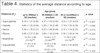
With the exception of the distances: lateral orbit, zygomatic arch; supra-
glenoid; gonion and supra M2 that had higher averages in females than in males.
For the others, the average measures were correspondingly higher in males.
However, there is significant differences between the sexes
(p<0.05) in the distances nasion, rhinion, midphiltrum,
supradentale and lateral orbit (Table 3).
Table 3 - Statistics of the averages of the distances according to sex.
| |
Sex |
| Distances (Di)
|
Male
Mean ± SD (median)
|
Female
Mean ± SD (median)
|
p Value
|
Distances (Di)
|
| • Supra-glabella |
4.34 ± 1.20 (4.13) |
4.10 ± 1.17 (4.17) |
4.25 ± 1.19 (4.16) |
p(1) = 0.528
|
| • Glabella |
4.92 ± 1.40 (5.03) |
4.82 ± 1.35 (4.61) |
4.88 ± 1.38 (4.88) |
p(2) = 0.733
|
| • Nasion |
6.12 ± 1.91 (6.15) |
5.19 ± 1.55 (5.09) |
5.76 ± 1.83 (5.81) |
p(1) = 0.011*
|
| • Rhinion |
4.73 ± 2.40 (4.12) |
3.20 ± 1.96 (2.71) |
4.14 ± 2.35 (3.42) |
p(1) < 0.001*
|
| • Midphiltrum |
14.29 ± 2.69 (13.94) |
11.32 ± 2.68 (11.46) |
13.14 ± 3.04 (13.30) |
p(2) < 0.001*
|
| • Supradentale |
11.81 ± 2.34 (11.94) |
9.16 ± 2.26 (8.73) |
10.79 ± 2.64 (10.50) |
p(2) < 0.001*
|
| • Infradentale |
10.29 ± 2.70 (10.00) |
9.65 ± 2.11 (9.48) |
10.05 ± 2.50 (9.72) |
p(1) = 0.178
|
| • Supramentale |
12.33 ± 2.38 (12.25) |
11.58 ± 2.45 (11.80) |
12.04 ± 2.42 (12.13) |
p(2) = 0.133
|
| • Pogonion |
11.10 ± 2.65 (11.26) |
10.44 ± 2.64 (10.00) |
10.84 ± 2.65 (10.80) |
p(2) = 0.228
|
| • Menton |
7.23 ± 2.73 (6.75) |
6.93 ± 2.72 (6.49) |
7.11 ± 2.72 (6.61) |
p(1) = 0.725
|
| • Supra-orbital |
6.34 ± 1.86 (6.19) |
6.23 ± 1.77 (6.20) |
6.29 ± 1.82 (6.19) |
p(2) = 0.773
|
| • Infra-orbital |
6.38 ± 2.46 (5.80) |
5.83 ± 2.18 (5.29) |
6.16 ± 2.36 (5.67) |
p(1) = 0.289
|
| • Lateral orbit |
7.20 ± 2.33 (7.06) |
8.81 ± 2.99 (8.65) |
7.82 ± 2.71 (7.42) |
p(3) = 0.006*
|
| • Inferior malar |
12.66 ± 3.73 (12.11) |
12.25 ± 4.71 (11.67) |
12.50 ± 4.12 (11.95) |
p(1) = 0.443
|
| • Zygomatic arch |
7.29 ± 2.52 (7.47) |
8.53 ± 3.06 (7.64) |
7.77 ± 2.79 (7.57) |
p(1) = 0.078
|
| • Supra-glenoid |
10.26 ± 3.84 (10.07) |
10.96 ± 3.78 (11.53) |
10.53 ± 3.81 (10.36) |
p(2) = 0.377
|
| • Gonion |
16.00 ± 6.38 (15.37) |
18.02 ± 6.98 (18.08) |
16.78 ± 6.66 (15.85) |
p(1) = 0.198
|
| • Supra M2 |
27.32 ± 5.77 (27.30) |
28.12 ± 6.24 (28.95) |
27.63 ± 5.94 (27.86) |
p(2) = 0.515
|
| • Occlusal line |
23.11 ± 4.42 (23.49) |
22.39 ± 4.52 (22.29) |
22.83 ± 4.45 (23.03) |
p(1) = 0.220
|
| • Sub M2 |
23.12 ± 4.84 (23.38) |
22.27 ± 5.46 (21.95) |
22.79 ± 5.08 (22.87) |
p(2) = 0.416
|
Table 3 - Statistics of the averages of the distances according to sex.
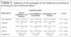
There were significant differences between categories of nutritional status for
the measures: glabella; nasion; pogonion; menton; supraorbital; lateral orbit;
inferior malar; supraglenoid; supra M2; occlusal line; sub M2 (Table 4). Most means grew with the
category of nutritional status, with higher measurements among overweighed
patients.
Table 4 - Statistics of the average distance according to age.
| Distances (Di)
|
Age group |
p value
|
up to 39
Mean ± SD (median)
|
40-59M
ean ± SD (median)
|
60 or more
Mean ± SD (median)
|
| • Supra-glabella |
4.19 ± 1.31 (4.08) |
4.37 ± 1.02 (4.40) |
4.23 ± 1.07 (4.03) |
p(1) = 0.801
|
| • Glabella |
4.60 ± 1.35 (4.64) |
5.29 ± 1.30 (5.49) |
5.18 ± 1.50 (4.59) |
p(1) = 0.056
|
| • Nasion |
5.59 ± 1.76 (5.51) |
6.22 ± 1.96 (6.06) |
5.37 ± 1.74 (5.25) |
p(2) = 0.213
|
| • Rhinion |
3.98 ± 2.37 (3.20) |
3.89 ± 1.62 (3.64) |
5.56 ± 3.40 (4.19) |
p(2) = 0.225
|
| • Midphiltrum |
13.74 ± 2.86 (13.70)(A) |
12.64 ± 3.11 (13.00)(AB) |
11.59 ± 3.20 (10.70)(B) |
p(3) = 0.043*
|
| • Supradentale |
11.16 ± 2.47 (11.01) |
10.52 ± 2.49 (10.50) |
9.68 ± 3.55 (8.66) |
p(1) = 0.165
|
| • Infradentale |
9.74 ± 2.54 (9.51) |
10.52 ± 2.31 (10.40) |
10.28 ± 2.74 (9.86) |
p(2) = 0.228
|
| • Supramentale |
12.15 ± 2.16 (12.20) |
11.91 ± 2.16 (11.95) |
11.88 ± 4.04 (11.93) |
p(1) = 0.876
|
| • Pogonion |
10.63 ± 2.57 (10.41) |
11.26 ± 2.79 (11.78) |
10.77 ± 2.77 (11.03) |
p(1) = 0.566
|
| • Menton |
6.43 ± 2.52 (6.02)(A) |
8.19 ± 2.68 (8.37)(B) |
7.61 ± 2.93 (7.67)(AB) |
p(2) = 0.011*
|
| • Supra-orbital |
5.95 ± 1.62 (5.70)(A) |
7.11 ± 1.91 (6.69)(B) |
5.85 ± 1.90 (6.28)(A) |
p(4) = 0.010*
|
| • Infra-orbital |
5.63 ± 2.15 (5.24)(A) |
6.92 ± 2.35 (6.52)(B) |
6.82 ± 2.86 (6.66)(AB) |
p(2) = 0.022*
|
| • Lateral orbit |
7.10 ± 2.34 (6.84)(A) |
8.84 ± 3.24 (8.47)(B) |
8.67 ± 1.85 (8.85)(AB) |
p(5) = 0.007*
|
| • Inferior malar |
12.12 ± 3.59 (11.88) |
13.58 ± 5.06 (13.90) |
11.54 ± 3.48 (12.29) |
p(2) = 0.394
|
| • Zygomatic arch |
7.59 ± 2.94 (7.28) |
8.24 ± 2.68 (7.66) |
7.45 ± 2.31 (7.59) |
p(2) = 0.439
|
| • Supra-glenoid |
9.68 ± 3.52 (9.96)(A) |
11.92 ± 3.57 (12.09)(B) |
11.04 ± 4.87 (9.39)(AB) |
p(1) = 0.025*
|
| • Gonion |
16.51 ± 6.29 (15.85) |
17.75 ± 6.75 (19.4) |
15.54 ± 8.28 (12.36) |
p(2) = 0.388
|
| • Supra M2 |
26.59 ± 5.47 (26.61) |
29.58 ± 5.47 (29.54) |
27.57 ± 8.19 (29.03) |
p(1) = 0.076
|
| • Occlusal line |
22.18 ± 4.37 (22.56) |
24.17 ± 4.45 (23.68) |
22.52 ± 4.43 (21.83) |
p(1) = 0.130
|
| • Sub M2 |
23.11 ± 4.52 (23.36) |
23.15 ± 5.89 (22.97) |
20.35 ± 5.10 (19.65) |
p(1) = 0.207
|
Table 4 - Statistics of the average distance according to age.
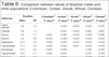
Tables 5 and 6 show results found in Brazilians compared to the ones in
other populations. Table 5 shows several
distances with significant differences (p < 0.05) when
considering males of each country: Colombians had nine distances; Koreans had
seventeen; Slovaks had thirteen; Africans had sixteen and Chinese had eleven
distances. Table 6 shows also many
distances with significant differences when considering females: Colombians had
ten distances; Koreans had twelve; Slovaks had nine; Africans had eleven and
Chinese had eight distances.
Table 5 - Statistics of the averages of the distances according to according to
the nutritional status.
| Distances (Di)
|
Nutritional status |
p value
|
Normal weight
Mean ± SD
(median)
|
Overweight
Mean ± SD (median)
|
Obesity
Mean ± SD (median)
|
| • Supra-glabella |
4.20 ± 1.20 (4.11) |
4.19 ± 1.14 (4.14) |
4.95 ± 1.27 (4.90) |
p(1) = 0.304
|
| • Glabella |
4.58 ± 1.30 (4.61)(A) |
5.06 ± 1.34 (5.09)(A) |
6.45 ± 1.05 (6.51)(B) |
p(2) = 0.001*
|
| • Nasion |
5.38 ± 1.68 (5.50)(A) |
5.91 ± 1.39 (6.02)(A) |
8.08 ± 3.17 (7.37)(B) |
p(3) = 0.001*
|
| • Rhinion |
4.29 ± 2.69 (3.25) |
4.07 ± 1.92 (3.85) |
3.22 ± 0.93 (3.20) |
p(1) = 0.622
|
| • Midphiltrum |
12.98 ± 3.20 (12.76) |
13.31 ± 2.96 (13.73) |
13.64 ± 2.30 (13.30) |
p(2) = 0.800
|
| • Supradentale |
10.39 ± 2.76 (10.02) |
11.42 ± 2.40 (11.57) |
1.85 ± 2.48 (11.00) |
p(2) = 0.185
|
| • Infradentale |
9.88 ± 2.55 (9.54) |
10.11 ± 2.62 (9.66) |
11.05 ± 0.84 (10.96) |
p(1) = 0.099
|
| • Supramentale |
12.01 ± 2.36 (12.15) |
12.16 ± 2.63 (12.04) |
11.69 ± 2.09 (12.20) |
p(2) = 0.890
|
| • Pogonion |
9.94 ± 2.42 (9.80)(A) |
12.06 ± 2.59 (12.32)(B) |
12.06 ± 1.95 (12.72)(B) |
p(3) < 0.001*
|
| • Menton |
6.22 ± 2.47 (5.57)(A) |
8.14 ± 2.41 (7.96)(B) |
9.19 ± 3.52 (10.40)(B) |
p(1) = 0.001*
|
| • Supra-orbital |
5.82 ± 1.62 (5.85)(A) |
6.63 ± 1.86 (6.31)(A) |
8.50 ± 1.24 (8.86)(B) |
p(3) < 0.001*
|
| • Infra-orbital |
5.93 ± 2.53 (5.43) |
6.28 ± 2.11 (5.84) |
7.56 ± 1.77 (7.23) |
p(1) = 0.077
|
| • Lateral orbit |
7.37 ± 2.49 (6.95)(A) |
8.14 ± 2.93 (7.57)(AB) |
9.92 ± 2.44 (9.07)(B) |
p(3) = 0.041*
|
| • Inferior malar |
11.70 ± 3.76 (10.85)(A) |
12.89 ± 4.27 (12.17) (A) |
17.07 ± 3.20 (16.83)(B) |
p(1) = 0.004*
|
| • Zygomatic arch |
7.45 ± 2.68 (7.45) |
7.89 ± 2.95 (7.47) |
9.78 ± 2.22 (10.86) |
p(1) = 0.070
|
| • Supra-glenoid |
9.70 ± 3.67 (9.89)(A) |
11.32 ± 3.90 (10.35)(AB) |
13.31 ± 2.52 (12.17)(B) |
p(1) = 0.018*
|
| • Gonion |
16.25 ± 6.64 (15.70) |
17.45 ± 6.60 (16.95) |
17.66 ± 7.71 (15.08) |
p(1) = 0.623
|
| • Supra M2 |
26.28 ± 5.57 (26.49)(A) |
28.99 ± 6.23 (29.24)(AB) |
31.77 ± 4.11 (31.90)(B) |
p(3) = 0.014*
|
| • Occlusal line |
21.37 ± 4.36 (21.28)(A) |
24.14 ± 3.54 (23.67)(B) |
28.15 ± 3.57 (27.07)(C) |
p(3) < 0.001*
|
| • Sub M2 |
21.71 ± 4.99 (21.23)(A) |
24.00 ± 5.06 (24.90)(B) |
25.48 ± 3.85 (24.13)(B) |
p(4) = 0.035*
|
Table 5 - Statistics of the averages of the distances according to according to
the nutritional status.
Table 6 - Comparison between values of Brazilian males and other populations
(Colombian, Corean, Slovak, African, Chinese).
| Distances |
Brazilian♂ |
Colombian2♂
|
Korean3♂
|
Slovak4♂
|
African5♂
|
Chinese6♂
|
| Mean |
DP |
P value(1) |
P value(1) |
P value(1) |
P value(1) |
P value(1) |
| Supra-glabella |
4.4 |
1.2 |
** |
<0.001* |
<0.001* |
<0.001* |
0.076 |
| Glabella |
4.6 |
1.2 |
** |
0.035* |
<0.001* |
0.002* |
0.987 |
| Nasion |
6.0 |
1.7 |
0.001* |
0.248 |
<0.001* |
< 0.001* |
0.898 |
| Rhinion |
5.2 |
2.8 |
<0.001* |
< 0.001* |
<0.001* |
<0.001* |
<0.001* |
| Midphiltrum |
14.7 |
2.6 |
0.424 |
<0.001* |
0.010* |
<0.001* |
<0.001* |
| Supradentale |
11.7 |
2.6 |
0.936 |
0.704 |
0.001* |
<0.001* |
<0.001* |
| Infradentale |
10.1 |
2.6 |
0.003* |
<0.001* |
** |
0.706 |
<0.001* |
| Supramentale |
12.5 |
2.1 |
0.932 |
0.019* |
** |
0.279 |
<0.001* |
| Pogonion |
10.2 |
2.4 |
** |
0.001* |
** |
<0.001* |
0.773 |
| Menton |
6.3 |
2.5 |
<0.001* |
0.030* |
** |
0.076 |
0.106 |
| Supra-orbital |
5.9 |
1.5 |
0.026* |
0.001* |
<0.001* |
0.001* |
0.001* |
| Infra-orbital |
6.3 |
2.8 |
0.011* |
0.002* |
0.051 |
0.231 |
0.072 |
| Lateral orbit |
7.0 |
2.4 |
0.031 |
<0.001* |
<0.001* |
0.322 |
<0.001* |
| Inferior malar |
11.9 |
3.0 |
<0.001* |
<0.001* |
<0.001* |
< 0.001* |
** |
| Zygomatic arch |
7.1 |
2.5 |
0.039* |
0.014* |
<0.001* |
<0.001* |
0.001* |
| Supra-glenoid |
9.4 |
3.7 |
0.207 |
<0.001* |
<0.001* |
0.020* |
0.034* |
| Gonion |
15.9 |
6.9 |
0.475 |
0.040* |
** |
0.030* |
0.052 |
| Supra M2 |
26.4 |
5.5 |
0.007* |
0.112 |
<0.001* |
< 0.001* |
0.325 |
| Occlusal line |
21.9 |
4.6 |
0.220 |
0.710 |
<0.001* |
<0.001* |
0.001* |
| Sub M2 |
23.0 |
4.9 |
0.194 |
0.002* |
** |
< 0.001* |
<0.001* |
Table 6 - Comparison between values of Brazilian males and other populations
(Colombian, Corean, Slovak, African, Chinese).
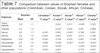
Table 7 shows the differences between
individuals overweighed of Brazil, China and Colombia. It shows significant
differences in 10 points in Chinese males, nine in Colombian males and 4 in
Chinese females.
Table 7 - Comparison between values of Brazilian females and other populations
(Colombian, Corean, Slovak, African, Chinese).
| Distances |
Brazilian♀ |
Colombian2♀
|
Korean3♀
|
Slovak4♀
|
African5♀
|
Chinese6♀
|
| Mean |
DP |
P value(1) |
P value(1) |
P value(1) |
P value(1) |
P value(1) |
| Supra-glabella |
3.9 |
1.1 |
** |
0.001* |
0.011* |
< 0.001* |
0.523 |
| Glabella |
4.5 |
1.4 |
** |
0.032* |
0.003* |
0.001* |
0.886 |
| Nasion |
4.6 |
1.3 |
<0.001* |
0.401 |
<0.001* |
0.149 |
0.001* |
| Rhinion |
3.0 |
1.9 |
0.003* |
0.003* |
0.001* |
0.213 |
0.164 |
| Midphiltrum |
10.8 |
2.6 |
<0.001* |
0.156 |
0.016* |
0.007* |
0.146 |
| Supradentale |
8.6 |
1.9 |
0.008* |
0.049* |
<0.001* |
<0.001* |
<0.001* |
| Infradentale |
9.6 |
2.5 |
0.012* |
<0.001* |
** |
< 0.001* |
<0.001* |
| Supramentale |
11.4 |
2.5 |
<0.001* |
0.001* |
** |
0.770 |
0.001* |
| Pogonion |
9.6 |
2.5 |
** |
0.001* |
** |
0.054 |
0.513 |
| Menton |
6.1 |
2.5 |
<0.001* |
0.945 |
** |
0.330 |
0.617 |
| Supra-orbital |
5.7 |
1.8 |
0.960 |
0.547 |
0.001* |
0.140 |
0.072 |
| Infra-orbital |
5.4 |
2.1 |
0.194 |
<0.001* |
0.008* |
0.109 |
0.053 |
| Lateral orbit |
7.8 |
2.6 |
0.011* |
0.006* |
0.017 |
0.298 |
0.001* |
| Inferior malar |
11.5 |
4.7 |
<0.001* |
<0.001* |
<0.001* |
< 0.001* |
** |
| Zygomatic arch |
8.0 |
2.8 |
0.886 |
0.737 |
0.255 |
<0.001* |
<0.001* |
| Supra-glenoid |
10.1 |
3.6 |
0.381 |
0.688 |
0.374 |
< 0.001* |
0.543 |
| Gonion |
16.7 |
6.4 |
0.075 |
<0.001* |
** |
<0.001* |
0.008* |
| Supra M2 |
26.2 |
5.7 |
0.003* |
0.680 |
0.987 |
< 0.001* |
0.589 |
| Occlusal line |
20.7 |
4.0 |
0.817 |
0.109 |
0.771 |
0.142 |
<0.001* |
| Sub M2 |
20.0 |
4.7 |
0.446 |
0.030* |
** |
< 0.001* |
0.476 |
Table 7 - Comparison between values of Brazilian females and other populations
(Colombian, Corean, Slovak, African, Chinese).
DISCUSSION
Demands in civil and criminal areas involving corpses or skeletons’
identification are enormous. For this reason, the process by which it determines
a person’s identity is crucial in trying to prove that a dead individual is
really himself. For this facial reconstruction may be used when other
identification methods have failed2. An
image of the unknown dead is obtained based on average values of facial soft
tissue thickness obtained in particular populations that can allow the
recognition of an individual.
This study evaluated soft tissue thickness among a Brazilian population, based in
predefined craniometric points using CT scans, aiming to create a population
data for future facial reconstructions for identification of skeletal remains.
This is important because variations between different populations may be found
and may interfere in these reconstructions.
This research found three points presenting higher soft tissue thickness: supra
M2, occlusal line and sub-M2. The points that showed smaller thickness were
located in the frontal bone (supraglabella, glabella, nasion) and the nose
region (rhinion). The rhinion point was the thinner. In agreement to the
population compared in this study Colombian27, Korean28, Slovak1, African23 and Chinese22, the
greatest thickness of the soft tissue in these populations were also in the
cheek region and the narrowest in the forehead and nasal root area.
Therefore, this is the only agreement in view of finding several distances with
significant difference when comparing them. The distances found to be different
with a p < 0.05 in almost all populations were rhinion;
supradentale; infradentale; supra orbital; inferior malar and zygomatic arch.
For over weighted individuals the distances found to be different were rhinion;
supradentale; infradentale; infra orbital; lateral orbit and oclusal line.
In this study, female’s distances in points such as lateral orbit, zygomatic
arch; supra-glenoid; gonion and supra M2 had average thickness higher than in
males. The other average measurements were correspondingly higher in males.
Significant statistical differences were observed between sexes
(p<0.05) in distances nasion, rhinion, midphiltrum,
supradentale, and lateral orbit.
However, based on statistical analysis, only forth of the thickness measurements
of the soft tissues of these anthropological marks were significantly different
between men and women. The same difference between sexes was found in the
Chinese population22, men had thicker
soft tissue than women in most points of reference, similar to other
populations23,27,28. A study on Slovakia population1 showed that soft tissue thickness of men’s face exceeded
females’ in 13 reference points, with 9 points with significant difference
(p < 0.05). Men showed higher values in points: lower
malar, occlusal line and upper M2.
Among the age groups (Table 8)
significant differences were recorded (p < 0.05) in
measures: midphiltrum; menton; supra-orbital; infra-orbital; lateral orbit;
supra-glenoid. According to Panenková1, in
Slovak population, men differ between the three age groups in supraglenoid point
and midphiltrum. Soft tissue thickness in females differed significantly in the
glabella, midphiltrum, supra-orbital and infra-orbital. Therefore, soft tissue
thickness might be different when comparing age groups.
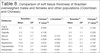
Table 8 - Comparison of soft tissue thickness of Brazilian overweighed males
and females and other populations (Colombian and Chinese).
| Distances |
Brazilian♂ |
Chinese2♂
|
Colombian3♂
|
Brazilian4♀
|
Chinese2♀
|
| Mean |
DP |
P value(1) |
|
Mean |
DP |
P value(1) |
| Supra-glabella |
4.3 |
1.2 |
0.009* |
** |
4.4 |
1.2 |
0.330 |
| Glabella |
5.3 |
1.5 |
0.138 |
** |
5.3 |
1.1 |
0.220 |
| Nasion |
6.3 |
2.1 |
0.208 |
0.310 |
6.2 |
1.5 |
0.638 |
| Rhinion |
4.2 |
1.7 |
0.009* |
<0.001* |
3.5 |
2.1 |
0.422 |
| Midphiltrum |
13.9 |
2.8 |
0.033* |
0.084 |
12.3 |
2.7 |
0.147 |
| Supradentale |
11.9 |
2.1 |
<0.001* |
0.028* |
10.1 |
2.6 |
0.002* |
| Infradentale |
10.5 |
2.8 |
<0.001* |
0.001* |
9.6 |
1.3 |
< 0.001* |
| Supramentale |
12.2 |
2.7 |
0.088 |
0.585 |
11.9 |
2.3 |
0.135 |
| Pogonion |
12.1 |
2.6 |
0.009* |
** |
11.9 |
2.4 |
0.063 |
| Menton |
8.3 |
2.6 |
0.166 |
<0.001* |
8.3 |
2.6 |
0.703 |
| Supra-orbital |
6.8 |
2.1 |
0.021* |
0.122 |
7.1 |
1.3 |
0.651 |
| Infra-orbital |
6.5 |
2.1 |
<0.001* |
0.021* |
6.5 |
2.2 |
0.034* |
| Lateral orbit |
7.4 |
2.3 |
<0.001* |
0.007* |
10.6 |
2.9 |
0.190 |
| Inferior malar |
13.5 |
4.3 |
** |
<0.001* |
13.6 |
4.6 |
** |
| Zygomatic arch |
7.6 |
2.5 |
0.358 |
0.008* |
9.5 |
3.3 |
0.089 |
| Supra-glenoid |
11.3 |
3.6 |
0.468 |
0.387 |
12.4 |
3.7 |
0.056 |
| Gonion |
16.1 |
5.8 |
0.566 |
<0.001* |
20.4 |
7.6 |
0.136 |
| Supra M2 |
28.4 |
5.9 |
0.330 |
0.131 |
31.6 |
5.7 |
0.349 |
| Occlusal line |
24.5 |
3.8 |
0.044* |
0.409 |
25.4 |
3.9 |
0.017* |
| Sub M2 |
23.2 |
4.9 |
0.598 |
0.286 |
26.4 |
4.3 |
0.061 |
Table 8 - Comparison of soft tissue thickness of Brazilian overweighed males
and females and other populations (Colombian and Chinese).
According to BMI, the measurement with significant differences were glabella;
nasion; pogonion; menton; supra-orbital; lateral orbit; inferior malar;
supra-glenoid; supra M2; occlusal line; sub M2, with lower soft tissue value
when the patient was normal followed by over weighted patients. In Chinese
population22 for both sexes, when
considering individuals overweighed, less distances had significant differences
when comparing to those with normal weight.
On the other hand, Colombians over weighted males had around half the amount of
distances with a significant difference, maybe because this study had a small
sample. Thus, it is possible to say that, when comparing populations between
them, BMI may be an important variable to consider since the differences tend to
diminish as the weight increases. However, since there is only these three
populations considering this variable, one of them with small samples
(Colombian/30 individuals)27, further
studies must be taken in order to study this issue more profoundly.
Some anthropometric points showed significant differences between sex, age groups
and nutritional status. Between sexes, men had greater means. Among age groups,
there was also significant differences in some distances. In relation to
nutritional status, the distances were lower among normal weight and higher
among the obese. When considering various populations, soft tissue thickness had
significant differences in many craniometric points highlighting how distinct
they might be.
CONCLUSION
Some anthropometric points showed significant differences between sex, age groups
and nutritional status. Between sexes, men had greater means. Among age groups,
there was also significant differences in some distances. In relation to
nutritional status, the distances were lower among normal weight and higher
among the obese. When considering various populations, soft tissue thickness had
significant differences in many craniometric points highlighting how distinct
they might be.
ACKNOWLEDGMENTS
This research received financial support from FACEPE, under a public call number
APQ-0150-4.02/14.
COLLABORATIONS
|
MMFS
|
Data curation; writing - original draft preparation.
|
|
GGP
|
Analysis and/or data interpretation; conception and design study;
final manuscript approval; methodology; project administration;
resources; writing - review & editing.
|
|
AAA
|
Conception and design study; conceptualization.
|
|
EPS
|
Conception and design study; supervision.
|
|
MVDC
|
Conceptualization; supervision.
|
|
RSCS
|
Conception and design study; methodology; supervision; writing -
review & editing.
|
REFERENCES
1. Panenková P, Beňuš R, Masnicová S, Obertová Z, Grunt
J. Facial soft tissue thicknesses of the mid-face for Slovak population.
Forensic Sci Int. 2012;220(1-3):293.e1-6.
2. Sipahioglu S, Ulubay H, Diren HB. Midline facial soft tissue
thickness database of Turkish population: MRI study. Forensic Sci Int.
2012;219(1-3):282.e1-8.
3. Manhein MH, Listi GA, Barsley RE, Musselman R, Barrow NE, Ubelaker
DH. In vivo facial tissue depth measurements for children and adults. J Forensic
Sci. 2000;45(1):48-60.
4. Stephan CN. Beyond the sphere of the English facial approximation
literature: ramifications of German papers on western method concepts. J
Forensic Sci. 2006;51(4):736-9.
5. Simpson E, Henneberg M. Variation in soft-tissue thicknesses on the
human face and their relation to craniometric dimensions. Am J Phys Anthropol.
2002;118(2):121-33.
6. Domaracki M, Stephan CN. Facial soft tissue thicknesses in
Australian adult cadavers. J Forensic Sci. 2006;51(1):5-10.
7. Codinha S. Facial soft tissue thicknesses for the Portuguese adult
population. Forensic Sci Int. 2009;184(1-3):80.e1-7.
8. Tedeschi-Oliveira SV, Melani RF, de Almeida NH, de Paiva LA. Facial
soft tissue thickness of Brazilian adults. Forensic Sci Int.
2009;193(1-3):127.e1-7.
9. Garlie TN, Saunders SR. Midline facial tissue thicknesses of
subadults from a longitudinal radiographic study. J Forensic Sci.
1999;44(1):61-7.
10. George RM. The lateral craniographic method of facial
reconstruction. J Forensic Sci. 1987;32(5):1305-30.
11. Smith SL, Buschang PH. Midsagittal facial tissue thicknesses of
children and adolescents from the Montreal growth study. J Forensic Sci.
2001;46(6):1294-302.
12. Utsuno H, Kageyama T, Deguchi T, Yoshino M, Miyazawa H, Inoue K.
Facial soft tissue thickness in Japanese female children. Forensic Sci Int.
2005;152(2-3):101-7.
13. Utsuno H, Kageyama T, Uchida K, Yoshino M, Oohigashi S, Miyazawa H,
et al. Pilot study of facial soft tissue thickness differences among three
skeletal classes in Japanese females. Forensic Sci Int.
2010;195(1-3):165.e1-5.
14. De Greef S, Claes P, Vandermeulen D, Mollemans W, Suetens P, Willems
G. Large-scale in-vivo Caucasian facial soft tissue thickness database for
craniofacial reconstruction. Forensic Sci Int. 2006;159 Suppl
1:S126-46.
15. Aulsebrook WA, Becker PJ, Iscan MY. Facial soft-tissue thicknesses
in the adult male Zulu. Forensic Sci Int. 1996;79(2):83-102.
16. El-Mehallawi IH, Soliman EM. Ultrasonic assessment of facial soft
tissue thicknesses in adult Egyptians. Forensic Sci Int.
2001;117(1-2):99-107.
17. Lebedinskaya GV, Veselovskaya EV. Ultrasonic measurements of the
thickness of soft facial tissue among the Bashkirs. Ann Acad Sci Fenn A.
1986;175:91-5.
18. Smith SL, Throckmorton GS. A new technique for three-dimensional
ultrasound scanning of facial tissues. J Forensic Sci.
2004;49(3):451-7.
19. Wilkinson CM. In vivo facial tissue depth measurements for white
British children. J Forensic Sci. 2002;47(3):459-65.
20. Vander Pluym J, Shan WW, Taher Z, Beaulieu C, Plewes C, Peterson AE,
et al. Use of magnetic resonance imaging to measure facial soft tissue depth.
Cleft Palate Craniofac J. 2007;44(1):52-7.
21. Sahni D, Sanjeev, Singh G, Jit I, Singh P. Facial soft tissue
thickness in northwest Indian adults. Forensic Sci Int.
2008;176(2-3):137-46.
22. Dong Y, Huang L, Feng Z, Bai S, Wu G, Zhao Y. Influence of sex and
body mass index on facial soft tissue thickness measurements of the northern
Chinese adult population. Forensic Sci Int.
2012;222(1-3):396.e1-7.
23. Phillips VM, Smuts NA. Facial reconstruction: utilization of
computerized tomography to measure facial tissue thickness in a mixed racial
population. Forensic Sci Int. 1996;83(1):51-9.
24. Kasai K. Soft tissue adaptability to hard tissues in facial
profiles. Am J Orthod Dentofacial Orthop. 1998;113(6):674-84.
25. Suzuki K. On the thickness of the soft tissue parts of the Japanese
face. J Anthropol Soc Nippon. 1948;60:7-11.
26. Rhine JS, Campbell HR. Thickness of facial tissues in American
blacks. J Forensic Sci. 1980;25(4):847-58.
27. Perlaza Ruiz NA. Facial soft tissue thickness of Colombian adults.
Forensic Sci Int. 2013;229(1-3):160.e1-9.
28. Hwang HS, Park MK, Lee WJ, Cho JH, Kim BK, Wilkinson CM. Facial soft
tissue thickness database for craniofacial reconstruction in Korean adults. J
Forensic Sci. 2012;57(6):1442-7.
29. Vanezi P, Vanezis M, McCombe G, Niblett T. Facial reconstruction
using 3-D computer graphics. Forensic Sci Int.
2000;108(2):81-95.
1. Universidade de Pernambuco, Camaragibe, PE,
Brazil.
Corresponding author: Gabriela Granja Porto, Av. General Newton
Cavalcanti, nº1650 - Camaragibe, PE, Brazil, Zip Code 54753-220. E-mail:
gabriela.porto@upe.br
Article received: April 25, 2018.
Article accepted: October 1, 2018.
Conflicts of interest: none.